Navigation bar

Load Data

Cellar contains several test datasets, most of which were generated by the Human BioMolecular Atlas Program (HuBMAP). These can be loaded and then downloaded using the Export Session functionality. Datasets are organized by data type, data center, and tissue. Data types include scRNA-seq, CODEX, scATAC-seq, SNARE-seq, etc, while tissues include lymph, spleen, thymus, kidney, heart, and more. Any uploaded datasets will appear first on the list.

For a list of accepted file formats check File Formats.

After loading a dataset, Cellar will check if 2D embeddings or cluster assignments are present in the file (only when uploading an AnnData object). If any are found, they will be used to automatically populate the plot and other relevant menus.

Dual Mode

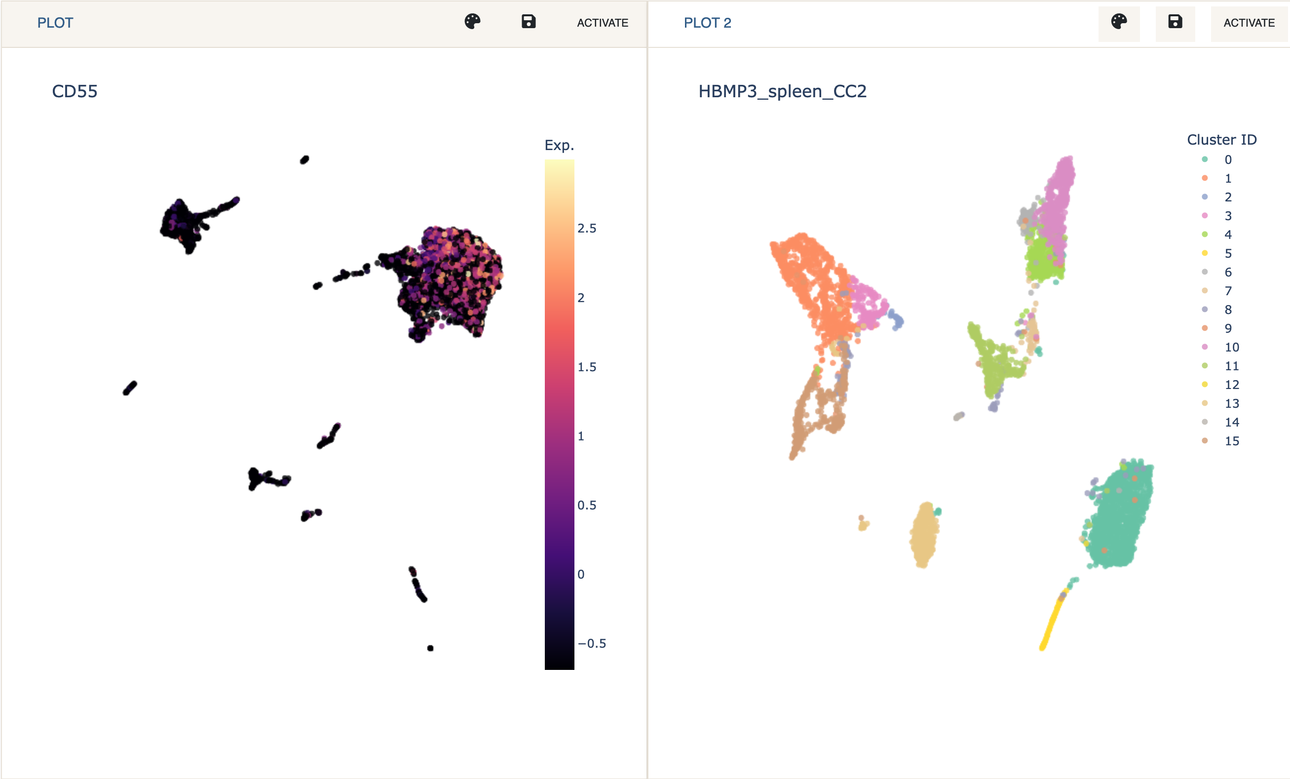
Dual Mode is used to analyze and visualize two datasets simultaneously. This can be particularly useful when analyzing SNARE-seq chromatin and mRNA expression data, or when integrating two datasets (e.g., via label transfer).

When in dual mode, only one dataset (plot) is active. This means that all of Cellar’s functionality applies to that dataset only. This includes clustering, annotation, and analysis panels. A plot can be activated by clicking the Activate button at that plot’s toolbar. Also, any label transfer functions assume the inactive dataset to be “reference” data, while the active dataset to be the one we wish to obtain labels for.

Dual Mode can be exitted by clicking Single View. This will not clear the session for the other plot and hitting Dual Mode again will recover the analysis.

Preprocessing

The preprocessing panel is split into two tabs. The first of these contains general preprocessing tools such as filtering cells or genes based on counts or normalizing each cell, while the second includes a special scATAC-seq preprocessing setup.

Preprocessing

The first panel uses the excellent preprocessing tools implemented in the scanpy Python package. Our choice of preprocessing options is guided by this tutorial. For a full description of the implemented preprocessing options consult scanpy’s API. Only the filters with checked boxes will be applied.

NOTE: All Server Datasets have been preprocessed using the default options. Therefore, there is no need to run preprocessing for these datasets and doing so might raise an error.

scATAC-seq

To allow the analysis of scATAC-seq data, we provide an option to convert a cell \(\small\times\) peak matrix to cell \(\small\times\) gene. This allows scATAC-seq data to be analyzed via the existing tools build in Cellar, just like you normally would with scRNA-seq data. The conversion is based on the open chromatin accessibility associated with the nearby region of all genes (as listed in GENCODE v35).

Formally, denote by \(P\in\mathbb{R}^{c\times p}\) the cell \(\small\times\) peak matrix and by \(G\in\mathbb{R}^{c\times n}\) the cell \(\small\times\) gene matrix to be created, where the total number of protein-coding genes in GENCODE v35 is \(n\). Fix \(j\in[n]\).

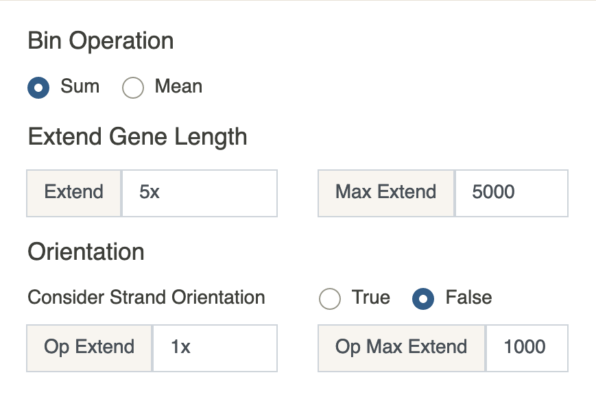
The first step is to extend the length of gene \(j\). Let the \(j^{\text{th}}\) gene location be the interval \(I_j=[\text{start}, \text{end}]\) where \(\text{start}\) and \(\text{end}\) are taken from GENCODE v35. We extend this interval by multiples of the gene length \((\text{end} - \text{start})\) or by a fixed number of base pairs. This value can be specified by the user in the Extend box. Any value that ends in x will be automatically considered a multiple of the gene length, otherwise it will be considered a fixed number of base pairs. Additionally, a Max Extend input box is provided which will limit the value of Extend. This is only useful when using a combination of gene length and a fixed number of base pairs.

Assume for convenience that Extend\(=5x\) and Max Extend\(=5000\). Then \(\text{start} \leftarrow \text{start} - \min(5\cdot(\text{end} - \text{start}), 5000)\). The same value is added to \(\text{end}\). If Consider strand orientation is set to Yes, you can specify different extension values to the end of the interval that corresponds to the downstream direction of the gene. This direction is determined by the strand key in the GENCODE v35 file.

Denote the updated interval by \(I_j^u\). The next step is to find peaks (bins) whose range intersects with \(I_j^u\). The values of these peaks are added or averaged (depending on the value of Operation to apply to bins) Formally, if we let \(K\) denote peak ranges, then

\(G_{i, j} = \text{op}(\{P_{i, k}: \text{for all } k \text{ such that } K_k \cap I_j^u \neq \emptyset\})\). The newly obtained cell \(\small\times\) gene matrix undergoes basic preprocessing and filtering just like in the previous tab.