Dimensionality Reduction
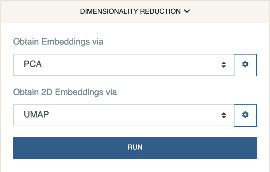
This panel is split into two select menus which contain almost the same set of dimensionality reduction methods. Cellar first reduces the data to a number of dimensions that is greater than 2. The goal is to denoise the data and obtain an embedding matrix that is more efficient to work with from a computational point of view. These embeddings are then further reduced to 2 dimensions for visualization purposes by using another (possible the same) method. By default, Cellar (but also other packages; e.g., Seurat, Scanpy), perform this two-step reduction by first applying Principal Component Analysis (PCA) followed by Uniform Manifold Approximation and Projection (UMAP).

-
Obtain Embeddings
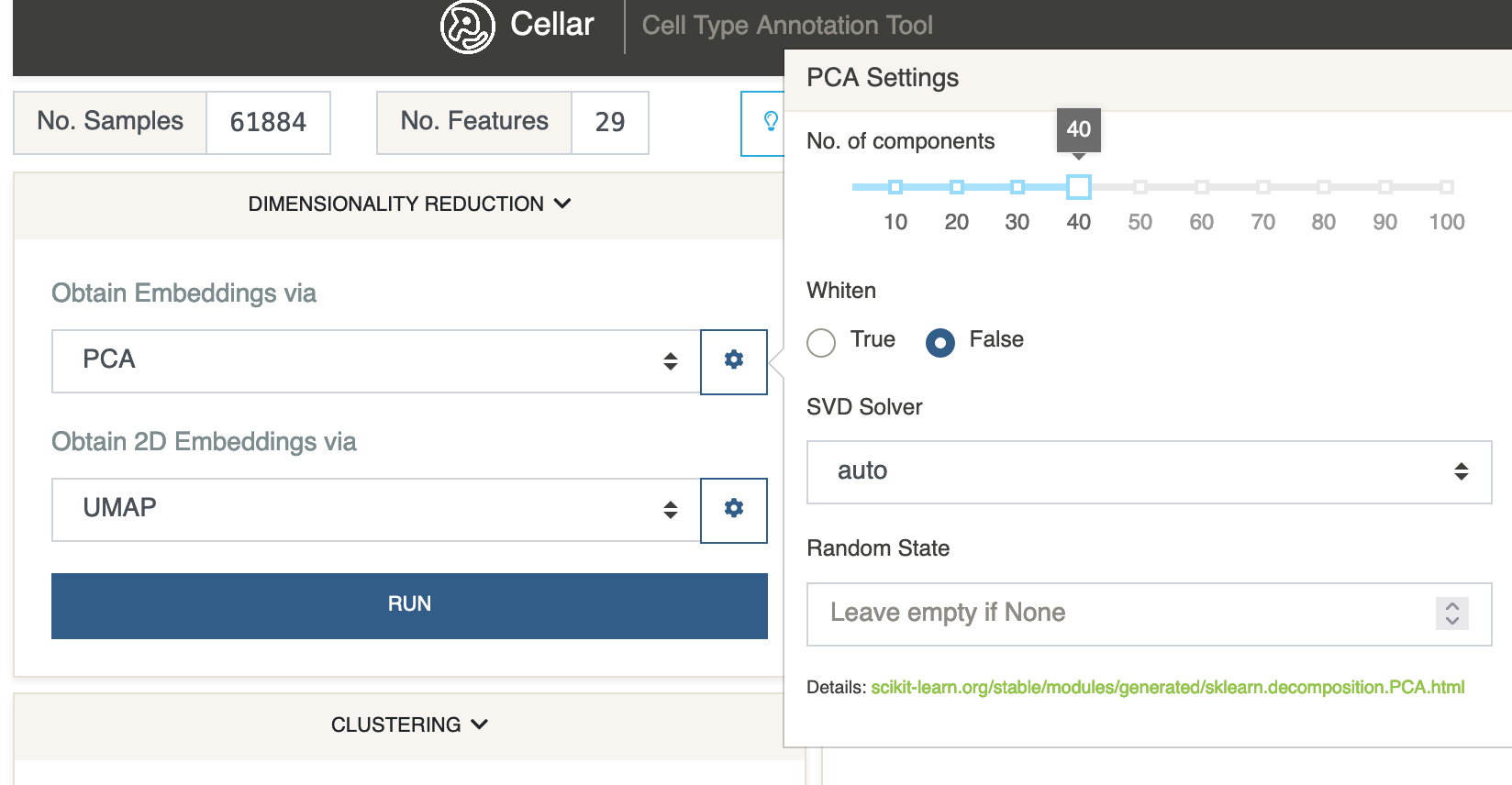
The default method is PCA with 40 principal components. PCA scales the data before computing the SVD, therefore, it cannot work with sparse matrices. If your data is sparse, Truncated SVD is a good alternative or even UMAP. PCA and Truncated SVD are typically the fastest performing methods from the list, with UMAP and Diffusion Maps being slower. cisTopic can be used when working with scATAC-seq data in cell-by-peak format. cisTopic will find cis-regulatory topics by using a probabilistic model based on Latent Dirichlet allocation, which can be interpreted as a reduced version of the data. This is quite useful in the case of scATAC-seq, since the number of peaks is typically a few hundred thousand and the data is very sparse which greatly harms the performance of other methods like PCA.
When working with CODEX data, it is common for the number of channels (proteins) profiled to be smaller than 40. In this case it may be necessary to reduce the default number of components from 40 to a smaller value. This can be achieved by clicking the gear-shaped button next to the menu which will expand various hyperparameters and settings related to the selected method.

-
Obtain 2D Embeddings
This list is almost the same as the previous one, with the addition of t-SNE. Typically UMAP gives the best results, with t-SNE being a close match. However, the time complexity of running t-SNE is quadratic which makes it much slower than UMAP. Furthermore, UMAP preserves more of the global structure than t-SNE, hence, it is the method we recommend for most cases. PCA can also be considered when a faster method than UMAP is desired. For some rough runtime estimates consult the bulb-shaped button next to the dataset’s shape.
Here is a nice tool you can use to gain a better understanding of how UMAP works.
A scatter plot of the 2D embeddings is shown after the dimensionality reduction step is complete. By default, all cells belong to a single cluster (ID 0).
The embeddings are stored in the anndata object under adata.obsm['x_emb'], while the 2D embeddings are stored under adata.obsm['x_emb_2d']. Relevant settings are stored under adata.uns['x_emb'] and adata.uns['x_emb_2d'].